Warning: this project was made some time ago, before I knew how to do Python properly. For example, the code snippets below inexplicably use camelCase. I have left the code unadulterated out of respect for my former naivity.#

If you’re still looking for this year’s boxing day project, I can recommend attempting to build your own physics engine from scratch. I set myself the goal of reaching the level of complexity required to simulate the mechanics of a pendulum clock. Here’s how it went.

Disclaimer#

This is not an exhaustive guide to coding, physics, or clocks. I’ve posted some code, and some equations, but these really only scratch the surface. Be aware that I mainly look at the physics problems here, when each of these presents several programming problems too. But if you are looking to do something similar, and just want a nudge in the right direction, then hopefully you will find this useful. I was only able to get anywhere by starting the simplest case and building up from there — and that’s exactly what this article does too.

The simulation environment#

It is tempting to dive straight in. But considering the environment variables at the outset will help us later, when things get more complicated.

Units#

• Objects will ultimately be drawn to a screen with pixel coordinates. We could use pixels as the unit of measurement, and this will work fine for standard translations in the x and y axis. But as soon as we start rotating objects, working with angles in radians and distance in pixels will get messy.
• If we instead denominate the simulation in SI units (ie metres, kilogrammes, Newtons), then equations of motion that handle torque (in Newton-metres), angular velocity (radians per second), and impulse (Newton-seconds) will work just fine.
• We will simulate objects in these units, and then convert to pixels in order to draw them to the screen. At the outset, then, we need functions to convert metres to pixels, and vice versa.

def metreToPixels(m):
    return m * constants.pixelsPerMetre

def metresToPixels(m):
    return [
        values.halfScreenPixelsX + metreToPixels(m[0]),
        values.halfScreenPixelsY - metreToPixels(m[1])
    ]

def pixelToMetre(p):
    return p / constants.pixelsPerMetre

def pixelsToMetres(p):
    return [
        -constants.screenMetres[0] / 2 + pixelToMetre(p[0]),
        constants.screenMetres[1] / 2 - pixelToMetre(p[1])
    ]

Sim time#

We want the simulation to run forwards (and maybe backwards) in time, but not necessarily at a fixed rate. So sim speed should be a variable. However, in order to maintain the consistency of the simulation at different speeds, we actually need three variables.

• Fps — frames per second drawn to the screen
• Sim multiple — how many sim iterations will run per frame draw
• Speed — how quickly, relative to normal time, the simulation will run

TICK = 60
SIM_MULTIPLIER = 2             # how many times the simulation runs per render tick
SPEED = 0.5                    # 1 = 100%

TIME_STEP = 1 / TICK / SIM_MULTIPLIER * SPEED       # seconds

def setTimeStep():
    return 1 / TICK / SIM_MULTIPLIER * SPEED

From these, we can derive the time step — or, how much time passes in each iteration of the simulation. For example, if we run the simulation 10 times per frame, at 60fps, and at 10% speed, then for each iteration of the simulation we will increment time by 0.00016666666 seconds. The smaller the time step, the more accurate certain elements of the simulation will be.

Being able to change these parameters while the simulation is running will enable easy debugging. If things are acting strangely, as they will very often, we can slow things right down to observe exactly what is going wrong. If we get really stuck investigating an inexplicable interaction, we can define an environment that reproduces the errant outcome and just keep slowing things down until we understand it.

The code environment#

import pygame

The environment variables above result in 600 iterations of the simulation per second. Performance is therefore quickly going to become a key consideration. While C++ would be an ideal choice of language, I chose to prototype in Python. This is because the project attempts to prove a concept, rather than result in production code. Python facilitates rapid prototyping, and modules such as Pygame give us a very easy way to draw to a screen, so that we can focus on the physics.

Counterintuitively, we can also see Python’s lack of performance as an advantage in the prototyping stage — it will be obvious to us which routines present speed bottlenecks, and which optimisations have a tangible effect.

Simulacra#

A ball#

Each object in the simulation will be an instance of an object in Python. All of the objects in our simulation will share certain characteristics, so we can declare those in a super-class called Object, of which Ball is a sub-class. Each object has its own draw function, where units are converted into pixels, and a call is made to the (very simple) Pygame draw function. Each type of object is likely going to require different physics models, so for now we can keep those particular to the sub-object.

class Object:

    def __init__(self, id, mass, CoM, angle, colour, hasGravity, canCollide, checkCollisions, fixed, root=None):

        self.id = id
        self.screen = constants.screen
        self.mass = mass
        self.CoM = CoM
        self.angle = angle
        self.colour = colour
        self.defaultColour = colour

        self.root = root
        if self.root == None:
            self.root = self.CoM

        self.hasGravity = hasGravity
        self.checkCollisions = checkCollisions
        self.canCollide = canCollide
        self.fixed = fixed

        self.velocity = [0.0, 0.0]
        self.angularVelocity = 0.0

        self.thrusts = []
        self.torques = []

        self.previousDistances = {}

        self.parent = None

    def getForces(self):
        return None

    def reset(self):
        self.thrusts = []
        self.torques = []


class Ball(Object):

    def __init__(self, id, CoM, radius, mass, colour, angle=0.0, hasGravity=True, canCollide=True, checkCollisions=True, calcPhysics=True, fixed=False):

        super().__init__(id=id, mass=mass, CoM=CoM, angle=angle, colour=colour, hasGravity=hasGravity, canCollide=canCollide, checkCollisions=checkCollisions, fixed=fixed)
        self.radius = radius
        self.radiusPixels = self.radius * constants.pixelsPerMetre
        self.MoI = physics.momentOfInertia(self, "circle")
        self.calcPhysics = calcPhysics

    def describe(self):
        print(f"CIRCLE -- id: {self.id}, centre: {self.CoM}, v: {self.velocity}, angle: {self.angle}, angleV: {self.angularVelocity}") 

    def draw(self):

        centrePixels = calc.metresToPixels(self.CoM)
        pygame.draw.circle(self.screen, self.colour, centrePixels, self.radiusPixels)

    def update(self):

        if self.calcPhysics:

            physics.applyForces(self)

            self.CoM[0] += self.velocity[0] * constants.TIME_STEP
            self.CoM[1] += self.velocity[1] * constants.TIME_STEP
            self.angle += self.angularVelocity * constants.TIME_STEP

Basic forces#

Let’s start out simple. If an object is accelerating due to gravity, then we can use simple equations of motion to find the acceleration of the object in each iteration of the simulation. Then we can add that acceleration to the object’s velocity vector, and move the object accordingly.

But in order to make the accuracy of our simulation independent of the time steps chosen, we can opt to calculate acceleration by solving the relevant differential equations. At this point we’re only interested in the acceleration due to gravity but we might as well include thrust forces and torques here now, as they will be useful later. This way we can have one physics function that will calculate acceleration due to all of the forces identified in the simulation.

def resultOfForces(object):

    def rb(y, t, g, m, thrusts, torques, I, k):
    
        vx, vy, theta = y

        # operate on list of forces
        if object.fixed == False:
            vx = (sum([T.vector[0] for T in thrusts]) - k * vx) / m
            vy = (sum([T.vector[1] for T in thrusts]) - m * g - k * vy) / m
        theta = (sum([np.cross(T.point, T.vector) for T in thrusts]) + sum(torques) - k * theta) / I

        dydt = [vx, vy, theta]
        
        return dydt

    y0 = [object.velocity[0], object.velocity[1], object.angularVelocity]

    timeStep = constants.TIME_STEP

    t = [0, timeStep]

    sol = odeint(rb, y0, t, args=(
        constants.GRAVITY if object.hasGravity else 0,
        object.mass,
        object.thrusts,
        object.torques,
        object.MoI,
        constants.FRICTION
    ))

    forces = {}

    forces["velocity"] = [sol[1][0], sol[1][1]]
    forces["angularVelocity"] = sol[1][2]

    return forces

Walls#

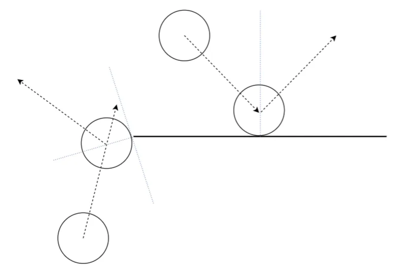
We are nearly ready to model our first interaction! Let’s start with a Ball v Wall collision, as this will allow us to take some considerable shortcuts. Assuming elasticity of 1 (no energy is “lost” during the collision), and no friction, a ball will simply be deflected by an immovable wall. We can therefore sidestep the physics for this case and instead invert the component of the ball’s velocity that is perpendicular to the wall.

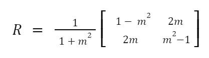
This will be trivial in the case of a vertical or horizontal wall, as in these cases the perpendicular component of the ball’s velocity is simply the x or y component of the vector. In other cases we must calculate the perpendicular component. Here we can make use of our first transformation matrix. All we need is m, the angle of the perpendicular to the line. Then we can reflect the ball’s velocity vector in the line given by gradient m using the following transformation matrix:

Transformation matrix for reflecting in a line given by gradient m

Collision detection#

In order to find m, we will need to properly detect a collision. From the ball’s perspective, this is pretty simple — if the distance to the wall is less than the radius of the ball, it has collided. But this begs the question — what is the distance to the wall?

Things are more complicated than they seem, as a ball can collide with a line in two ways:

• At one of the ends
• At some point between the ends

We can use trigonometry to calculate where the ball will collide. If angle a or b is greater than 90 degrees, the collision will occur at the respective end. If both a and b are less than 90 degrees, and the height of the triangle is less than than the radius of the circle, then the collision occurs somewhere in the middle.

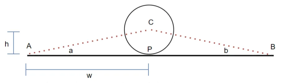
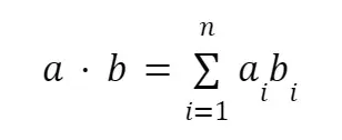
The exact point of collision P can be found by using trigonometry and Pythagoras’ theorem to solve for w. This process can be made computationally less intensive by instead projecting the vector AC onto the vector AB using the vector dot product, which gives the ratio of w to AB.

Dot product of vectors a and b gives the projection of a onto b

Having ruled out a midway collision, a collision with the end of a line is easy to detect. Since the end is a point, we can simply calculate the distance from the centre of the ball to that point. Reflecting the ball’s velocity in the line drawn between the end and the ball’s centre produces the expected behaviour.

Component of ball’s velocity perpendicular to approach is inverted

Ball v Ball#

Unfortunately, things get more complex from here. In order to accurately model collisions between two moving objects, we must conserve momentum and kinetic energy. The subsequent velocities depend on the initial velocities and masses of each of the colliders, and are given by:

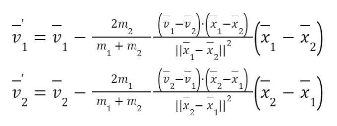
Where:

• v is velocity vector of each respective ball
• m is mass of each respective ball
• x is the position vector of each respective ball This can be implemented slightly more succinctly in code:

def circleCircleCollision(objectA, objectB, intercept, distance):

    n = [intercept[0] / distance, intercept[1] / distance]
    p = (2 * (dot(objectA.velocity, n) - dot(objectB.velocity, n))) / (objectA.mass + objectB.mass)

    pma = p * objectA.mass
    pmb = p * objectB.mass

    objectA.velocity = [objectA.velocity[0] - pmb * n[0], objectA.velocity[1] - pmb * n[1]]
    objectB.velocity = [objectB.velocity[0] + pma * n[0], objectB.velocity[1] + pma * n[1]]

At this point, we are checking every collidable object with every other collidable object, every iteration of the simulation. Optimisation strategies start to become important.

Beyond Balls#

If we want to move beyond modelling the interactions between balls, we can ignore angular velocity no longer. In order to simulate collisions that involve angular momentum, we must calculate the impulse imparted by the collision, and subsequently its effect on each of the colliders’ linear and angular velocity.

The equation we need for impulse j is:

Solving for impulse

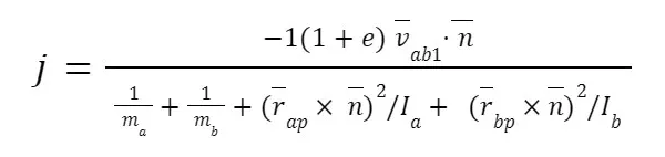
Where:

• e is elasticity (1 is perfectly elastic, 0 is completely inelastic)
• vab1 is the relative velocity with which the colliding points are approaching each other, taking into account linear and angular velocity (some linear algebra required to compute this)
• n is the vector normal to the edge of body b, of length 1
• r is the distance vector from the center of mass of a body to the collision point
• I is the moment of inertia of a body We can then use the impulse to solve for the final linear and angular velocities.

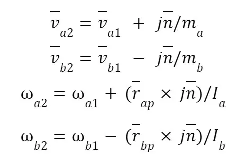
Where:

• w is the angular velocity of each body

This was not easy to get working properly. Below is a version of this formula implemented in code. This can be the base for other cases, such as those in which bodies are fixed in position about a freely rotating point.

def collision(objectA, objectB, pointA, pointB):

    AcomToPoint = getLineVector([objectA.root, pointA])
    BcomToPoint = getLineVector([objectB.root, pointB])

    # velocity of point = translational velocity vector + rotational velocity vector
    pointArotationalSpeed = norm(AcomToPoint) * objectA.angularVelocity
    perpRotationVector = calc.rotateVector(AcomToPoint, 270)
    pointArotationVector = calc.scaleVector(perpRotationVector, pointArotationalSpeed)

    pointBrotationalSpeed = norm(BcomToPoint) * objectB.angularVelocity
    perpRotationVector = calc.rotateVector(BcomToPoint, 270)
    pointBrotationVector = calc.scaleVector(perpRotationVector, pointBrotationalSpeed)

    relPointV = subVectors(
        addVectors(
            objectA.velocity, pointArotationVector
        ),
        addVectors(
            objectB.velocity, pointBrotationVector
        )
    )

    perpImpactVector = normaliseVector(getLineVector([pointB, pointA]))

    aTerm = squareVector(cross(AcomToPoint, perpImpactVector)) / objectA.MoI
    bTerm = squareVector(cross(BcomToPoint, perpImpactVector)) / objectB.MoI

    impulse = (
        dot(relPointV, perpImpactVector) * -(1 + constants.ELASTICITY) /
        (
            1 / objectA.mass + 1 / objectB.mass + aTerm + bTerm
        )
    )

    objectA.velocity = addVectors(objectA.velocity, scalarDiv(scalarMult(perpImpactVector, impulse), objectA.mass))
    objectB.velocity = addVectors(objectB.velocity, scalarDiv(scalarMult(perpImpactVector, -impulse), objectB.mass))
    objectA.angularVelocity += cross(AcomToPoint, scalarMult(perpImpactVector, impulse)) / objectA.MoI
    objectB.angularVelocity -= cross(BcomToPoint, scalarMult(perpImpactVector, impulse)) / objectB.MoI

Thrusts#

We’re now getting to the stage where we have the building blocks to be able to simulate more complex systems.

Remember the thrust term we included in the differential equation earlier? We can now use that to get objects to respond to any forces, such as that generated by a spring, or by user input. A spring simply adds thrusts to the things at either end, in proportion to the extent of its extension:

class Spring(Object):

    def __init__(self, id, objectA, objectB, strength, colour, canCollide=False):

        super().__init__(id=id, mass=0, CoM=[0,0], angle=0, colour=colour, hasGravity=False, canCollide=canCollide, checkCollisions=False, fixed=False)
        self.objectA = objectA
        self.objectB = objectB
        self.strength = strength
        self.widthPixels = 15

    def getForces(self):
        length = norm(calc.getLineVector([self.objectA.CoM, self.objectB.CoM]))
        springForce = physics.springForce(self.strength, length)

        thrustAVector = calc.getLineVector([self.objectA.CoM, self.objectB.CoM])
        thrustAVector = calc.scaleVector(thrustAVector, springForce)

        thrustBVector = calc.getLineVector([self.objectB.CoM, self.objectA.CoM])
        thrustBVector = calc.scaleVector(thrustBVector, springForce)

        self.objectA.thrusts.append(physics.Thrust(
            thrustAVector, [0,0]
        ))

        self.objectB.thrusts.append(physics.Thrust(
            thrustBVector, [0,0]
        ))

    def update(self):
        return None

    def draw(self):
        self.startPixels = calc.metresToPixels(self.objectA.CoM)
        self.endPixels = calc.metresToPixels(self.objectB.CoM)

        pygame.draw.line(self.screen, self.colour, self.startPixels, self.endPixels, round(self.widthPixels))

Systems#

We can also use what we have already built to define systems. Systems will be made up of objects such as lines and balls. The tremendous thing about using objects we’ve already made is that the collision detection already exists, and can be used without modification.

We just have to ensure that when a component is in a collision, the resolution is computed for the system as a whole. We achieve this by ensuring that the components inherit the mass, moment of inertia, and centre of mass of the whole. Then the results of the collision can be computed at the component level exactly as collisions between individual objects were, before being propagated to all children.

We also need some logic for calculating the moment of inertia of a system. In order to move the child objects around when the parent translates or rotates, some more linear algebra is needed. In order for systems to be able to swing around a fixed point, we also need to move the object’s centre of mass when it rotates.

class System(Object):

    def __init__(self, id, objects, root, CoM=None, angle=0, hasGravity=True, calcPhysics=True, fixed=True, sumMoI=True):

        mass = 0
        self.MoI = 0
        for object in objects:
            mass += object.mass
            if sumMoI:
                self.MoI += object.MoI
            else:
                # simple approximation of MoI - for lines only
                self.MoI += object.mass * norm(calc.getLineVector([root, calc.lineCentre(
                    [calc.addVectors(root, object.rootToStart),
                    calc.addVectors(root, object.rootToEnd)]
                )]))

        if CoM == None:
            # calculate CoM here if being fancy
            CoM = [0, 0]

        self.objects = objects
        self.fixed = fixed
        self.calcPhysics = calcPhysics

        super().__init__(id=id, mass=mass, root=root, CoM=CoM, angle=angle, colour="white", hasGravity=hasGravity, canCollide=False, checkCollisions=False, fixed=fixed)

        # if self.fixed:
        self.pivotCoMvector = calc.getLineVector([self.root, self.CoM])
        self.pivotRadius = norm(self.pivotCoMvector)

        # each object has same MoI and mass as parent
        # this means we don't have to change collision resolution much
        for object in self.objects:
            object.mass = self.mass
            object.MoI = self.MoI
            object.parent = self
            object.fixed = self.fixed

    def describe(self):
        print(f"SYSTEM -- id: {self.id}, centre: {self.CoM}, v: {self.velocity}, angle: {self.angle}, angleV: {self.angularVelocity}, objects: {self.objects}") 

    def getForces(self):

        self.torques.append(physics.swingTorque(self))

        # need to put torques on children for proper calculations in Contact
        for object in self.objects:
            object.torques = self.torques

    def update(self):

        # move up object model?
        if not(self.fixed):
            physics.applyForces(self)
            self.CoM[0] += self.velocity[0] * constants.TIME_STEP
            self.CoM[1] += self.velocity[1] * constants.TIME_STEP

            self.root = self.CoM
            self.angle -= self.angularVelocity * constants.TIME_STEP

        elif self.fixed:
            if self.calcPhysics:
                physics.applyForces(self)
                self.angle -= self.angularVelocity * constants.TIME_STEP
                self.updateCoM()

        for object in self.objects:
            object.root = self.root
            object.CoM = self.CoM
            object.angle = self.angle
            object.velocity = self.velocity
            object.angularVelocity = self.angularVelocity
            object.update()

        return None

    def updateCoM(self):

        # rotate CoM around pivot
        newVector = calc.rotateVector(self.pivotCoMvector, self.angle)
        self.CoM = [self.root[0] + newVector[0], self.root[1] + newVector[1]]

    def draw(self):

        return None

Swing Torque#

In the simulation above, the system rotating around a fixed point has an offset centre of mass — which results in a torque due to gravity. We’ll need to calculate this properly if we we want to simulate pendulum clocks, but that’s fortunately very simple. Force about the pivot due to gravity will be the component of gravitational force that is perpendicular to a hanging object’s tether (or the line from the centre of mass to the pivot point). This torque will then be collected by the differential equation solver we made earlier, which will find the acceleration in a given time step for a given object’s moment of inertia.

def swingTorque(object):

    if object.pivotRadius == 0:
        return 0

    pivotToCoM = getLineVector([object.root, object.CoM])
    angle = np.radians(270) - theta(pivotToCoM, [1, 0])
    force = constants.GRAVITY * np.sin(angle)
    torque = object.pivotRadius * force

    return torque

Contact forces#

When elasticity is 1, all of the energy in a collision is preserved in the final velocities. This means that objects will always be moving away from each other after a collision.

The closer elasticity gets to 0, the more objects will tend to penetrate one another unless additional forces are modelled. Contact force is the force that an objects impart on one another when at rest.

Below is the same setup as before, only with much lower elasticity. Things clip through the floor, and each other, because they lose energy upon collision. After collision, they have less kinetic energy in the opposite direction. Each time this cycle repeats, the distance between the objects will shrink — and there’s nothing to stop it becoming negative.

The solution to this is unfortunately quite complex, and involves carefully reworking the main simulation loop.

• In the collision detection loop, we must determine whether touching objects are colliding or merely in contact, based on closing speed of contact points. Above a certain threshold of perpendicular motion, objects will be said to collide. But if they are moving slowly enough, we resolve a contact instead. Defining this threshold is largely trial and error. As is efficiently measuring it.
• If objects are touching but not colliding, we need to calculate how much force each object requires in order to prevent it from accelerating into the other. This involves looking forward in time to the next update, and the relative future velocities of the collision points on the objects, based on the forces on them and the subsequent linear and angular acceleration. For this reason, the sim loop has to be reengineered to collect forces before implementing them. We then have to calculate how much force to apply to each object, and where, in order to neutralise the components of linear and angular velocity that are towards each other. If done correctly, this allows force to be transmitted between two stationary objects if, for example, one has a torque and the other has high inertia — as in the escapement of a clock. It should also allow objects to slide against one another while they resist penetration, since we only cancel the perpendicular component of the motion.

Implementing even a basic version of contact forces adds considerable computational overhead to the simulation, as we now have to solve the same differential equations twice — once for the current time step, and once for the next time step, in order to cancel a component of that acceleration. But, we can again make use of the existing mechanism for resolving thrusts, since a contact force will be felt perpendicular from the point of contact, and can be resolved in the next iteration.

Putting it all together#

We now have everything we need to simulate the escapement of a pendulum clock! We can define a pendulum and escapement system as a series of lines. Same for the gear wheel. In the pendulum/escapement’s case, we set the centre of mass waaaay below the pivot point. Our line-line collision detection will find interactions, which will then, thanks to the contact forces we’ve just modelled, result in torque in the gear being transferred into energy in the pendulum. We’ll assume that all parts except for the bob have negligible weight, meaning that the centre of mass is at the end of the pendulum, making the moment of inertia nice and easy to calculate.

Given how much linear algebra we’ve had to use for this project, it’s satisfying to be able to implement a quick shortcut for generating the toothed gear — all we need to do is rotate a tooth that is offset from its root a certain number of times around the centre.

teeth = []

for tooth in range(toothCount):

    angle = (np.radians(360) / toothCount) * tooth

    rootToStart = [0.15, 0]
    rootToStart = calc.rotateVector(rootToStart, angle)

    rootToEnd = [0.15, -0.232]
    rootToEnd = calc.rotateVector(rootToEnd, angle)

    tooth = objects.Line(
        id = objectCount,
        mass = 0.005,
        colour = "darkorange",
        root = gearCentre,
        rootToStart=rootToStart,
        rootToEnd=rootToEnd,
        width = 0.02,
        calcPhysics=True,
        canCollide=True,
        checkCollisions=False
    )
    objectCount += 1

    teeth.append(tooth)

Then we can add a function to the main sim loop that adds a small torque to the gear each iteration.

gearTorque = 0.05

def clock1Torque():
    physics.applyTorque(gearSystem, gearTorque)

constants.simIterationFunctions.append(clock1Torque)

Finally, we set elasticity to 0.25, to simulate most of the pendulum’s energy coming from contact forces rather than collision forces, as in real life. And then we set it running!

The result? Maths says that a pendulum of this length should oscillate with a period of around 2.3s, and this one has a period of around 2.1s.

From here, the sky is really the limit. Double pendulums, triple pendulums, polygons, and articulated connectors would all be obvious next steps. As would resolving contact forces simultaneously for all objects in a chain of contact.

But I’d call that good enough for now.