Pictionary with Recurrent Neural Networks
Objectives#
I wanted to train a neural network to recognise sketches made by a player with sufficient speed and accuracy to make a 1-player version of Pictionary possible. In order to create an experience analogous to 2-player Pictionary, I wanted to train a model capable of making accurate guesses using drawings at various stages of their completion. This article details that process.
TLDR You can play around with the game here: https://mrpickleapp.github.io/pictionary-game-js/
And you can find all the Python modelling and Javascript game code here: https://github.com/mrpickleapp/pictionary-game-js
The data#
Google has made 50 million drawings made in the Quick, Draw! game available to download. Of several file formats, I chose the custom .bin due to its smaller file size and efficient processing, though this necessitates a bespoke file parser. You can find all of Google’s documentation here.
Each drawing contains an array of strokes, which can be of varying length. Each stroke is also of varying length, and contains two tuples of x and y point coordinates, in the form:
((x1, x2, x3, …), (y1, y2, y3, …))
…such that the stroke can be plotted with (x1, y1), (x2, y2), (x3, y3), …
The raw data looks like this:
((157, 117, 51, 25, 17, 22, 27, 37, 40, 85, 148), (248, 250, 239, 226, 205, 184, 175, 169, 179, 194, 196))
((148, 148), (196, 196))
((114, 206, 215, 246, 255, 243, 214, 205, 195, 190, 104), (213, 183, 155, 127, 108, 93, 94, 99, 123, 126, 154))
((205, 213, 215), (98, 78, 63))
((121, 161, 174, 181, 179, 157, 132, 73, 38, 20, 8, 0, 0, 6, 19, 29, 35), (142, 106, 87, 65, 35, 12, 4, 0, 7, 16, 36, 75, 117, 137, 155, 165, 166))
((87, 88, 127, 128, 120, 101, 81, 63, 44, 36, 35, 44, 57, 76, 92, 103, 107, 104, 90, 85, 83, 85, 90, 101), (133, 124, 78, 56, 39, 29, 30, 35, 44, 72, 91, 107, 114, 115, 109, 99, 91, 65, 63, 66, 73, 78, 77, 66))
And when plotted, it looks like this:
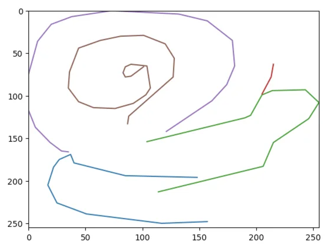
A few points about these points:
- The y-axis is inverted, with (0, 0) being the top left corner. This is the convention in computer graphics, so we’ll have to make sure we observe this consistently.
- Note that the drawing fills the canvas in the x-axis, and there is no padding on three sides. This is because the drawing has been rescaled to fill the frame, while maintaining aspect ratio.
- The points are sparser than you would expect from a human hand, resulting in long straight lines between them. This is because the drawings have been simplified using the Ramer-Douglas-Peucker algorithm.
After training the model, we will have to recreate these steps for new drawings in order to make accurate predictions.
Classifying incomplete drawings#
A design goal of this project is to have the AI guess in real-time. This means that we want to predict from the model after every stroke. This presents a couple of problems:
- If the model has only ever seen finished drawings, it likely won’t predict well from partial drawings.
- Incomplete drawings might be of very different scales, because the final drawings have been rescaled according to their final dimensions.
The solution to this is to include in the training set drawings at every stage of completion. If we treat each drawing-stage as a separate drawing, and rescale it accordingly, then we have a consistent mechanism for handling incomplete sketches. This should also help with overfitting, since:
- Despite showing the model the same strokes multiple times, they may appear in different places and at different scales.
- These incomplete drawings have high uncertainty associated with them, so also act like a form of noise. However, a more complete solution would involve adding noise (in the form of random positional adjustments, translations, rotations, aspect ratio changes, etc) to incomplete drawings to more fully address the potential for overfitting. Alternatively, we could include each drawing only once, picking a stage from it at random.
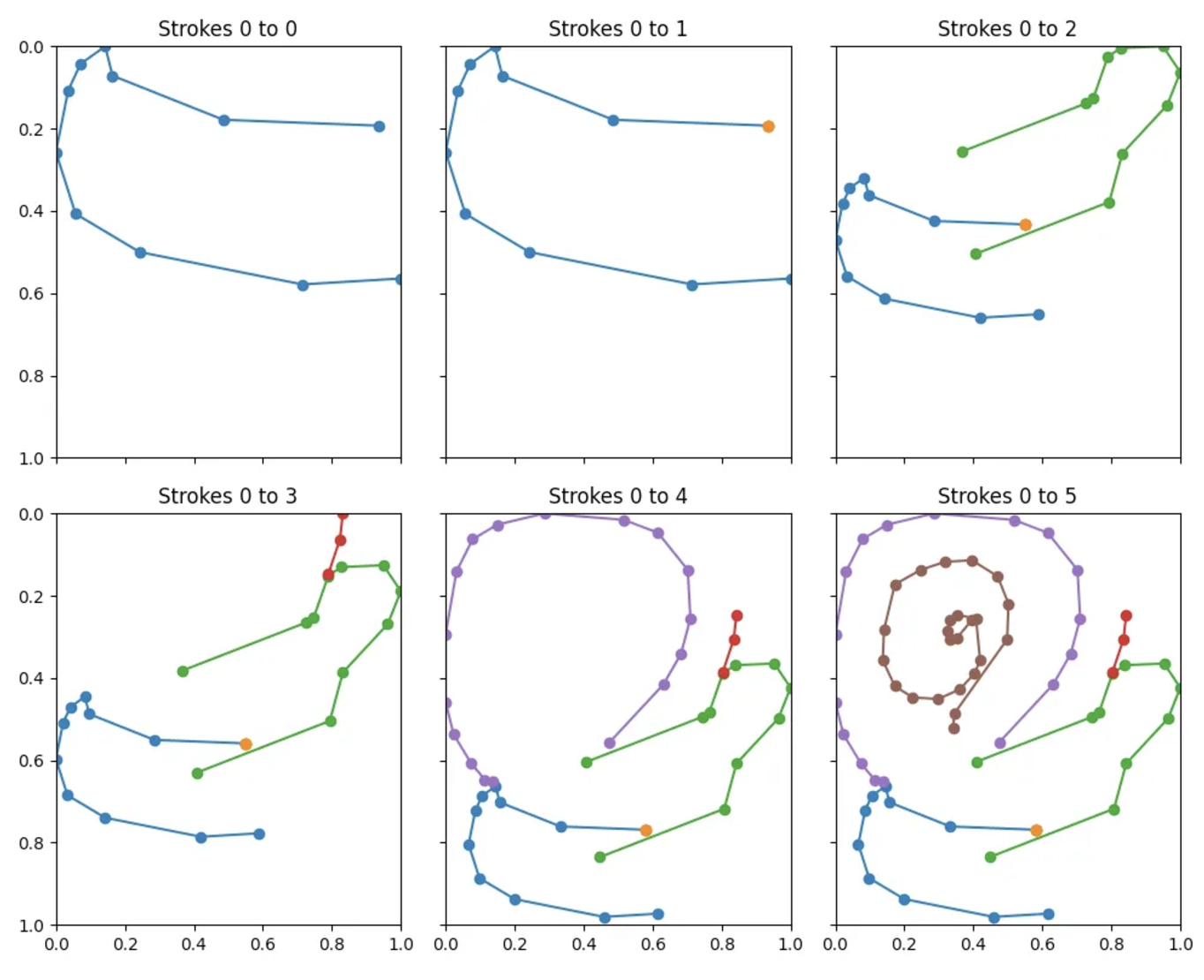
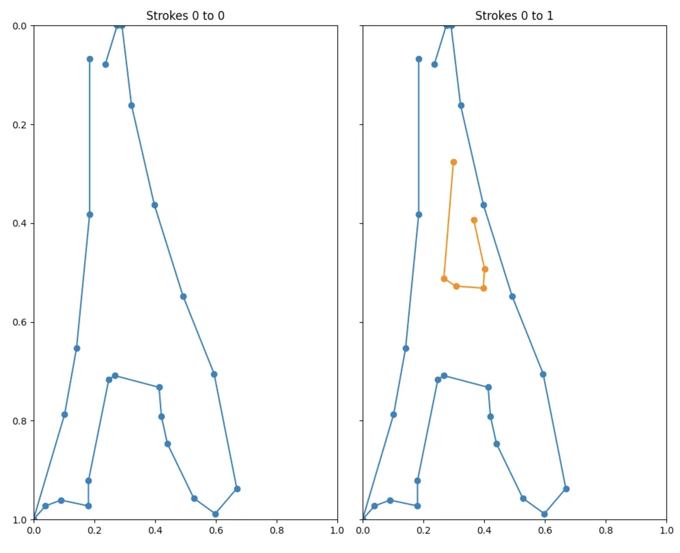
For the snail above, the first strokes are unlikely to prove instructive. For the Eiffel Tower below, though, stroke 0 should be enough to make a good prediction.
Input data#
One final layer of processing is required before the model can use this data.
- The strokes are scaled to a 0–1 range. This helps training but also provides a consistent base for building applications.
- The strokes are turned from points into deltas — or the change in x, y from the previous point.
- For each point, a binary flag indicates whether the point is the start of a new stroke.
- The data is padded with zeroes to a predefined length (in our case, there is a max of 200 points). This is because the neural network will expect inputs of consistent shape.
All of this means that the final form for each drawing is an array of shape (200, 3), where each row comprises [x, y, z], where -1 ≤ x ≤ 1, -1 ≤ y < 1, and z = 0 | 1.
array([[ 0.18503937,  0.06692913,  1.        ],
       [ 0.        ,  0.31496063,  0.        ],
       [-0.04330709,  0.27165354,  0.        ],
       [-0.03937008,  0.13385827,  0.        ],
       [-0.1023622 ,  0.21259843,  0.        ],
       [ 0.03937008, -0.02755906,  0.        ],
       [ 0.0511811 , -0.01181102,  0.        ],
       [ 0.09055118,  0.01181102,  0.        ],
       [ 0.        , -0.0511811 ,  0.        ],
       [ 0.06692913, -0.20472441,  0.        ],
       [ 0.01968504, -0.00787402,  0.        ],
       [ 0.14566929,  0.02362205,  0.        ],
        ...
The model#
I used a basic Recurrent Neural Network (RNN) for the following reasons:
Sequential Data Processing:#
- Sketches are inherently sequential. They are made up of a series of strokes, where each stroke consists of a sequence of points (x, y coordinates). RNNs are explicitly designed to handle sequential data.
Temporal Dependencies:#
- In sketching, the order of strokes and their relationship over time is crucial. RNNs can capture temporal dependencies, which means they remember previous strokes while processing new ones. This ability allows the network to understand and predict the continuation of a drawing based on its history.
Variable Sequence Length:#
- Drawings can have varying numbers of strokes and points. RNNs can handle sequences of different lengths, which is crucial for processing diverse sketches.
In order to train in a reasonable time on my meagre CPU, I kept things pretty simple.
def _build_model(self):
      model = tf.keras.models.Sequential()

      # Input layer
      model.add(tf.keras.layers.Input(shape=self.state_shape))

      # Masking layer
      model.add(tf.keras.layers.Masking(mask_value=0.))

      # 1D Convolutional Layers
      model.add(tf.keras.layers.Conv1D(32, 3, activation='relu'))
      model.add(tf.keras.layers.Conv1D(64, 3, activation='relu'))
      model.add(tf.keras.layers.MaxPooling1D(2))

      model.add(tf.keras.layers.Conv1D(128, 3, activation='relu'))
      model.add(tf.keras.layers.MaxPooling1D(2))

      # Recurrent layers (e.g., LSTM)
      model.add(tf.keras.layers.LSTM(128, return_sequences=True))
      model.add(tf.keras.layers.LSTM(128))

      # Dense layers
      model.add(tf.keras.layers.Dense(128, activation='relu'))
      model.add(tf.keras.layers.Dense(128, activation='relu'))

      # Output layer
      model.add(tf.keras.layers.Dense(self.num_categories, activation='softmax'))

      model.compile(loss='sparse_categorical_crossentropy', optimizer=tf.keras.optimizers.Adam(learning_rate=self.learning_rate), metrics=['accuracy'])

      return model
Training#
To keep training times reasonable, I trained this model on a subset of the full dataset. For each of the 345 categories, I added 4,096 examples to the training set and 1,024 to the validation set (remember that each drawing may appear in the set multiple times at various stages of completion). This makes a total of 1,413,120. With over 50m drawings in the full dataset, more compute time could clearly be of great benefit.
With the simple model above, a validation accuracy of around 0.6 was achieved after 10 epochs. Accuracy for complete drawings should be considerably higher.
Testing the model#
I initially wrote a simple Python script using the pygame module to test both the model and the image processing functions. In order to make a prediction from a drawing, we use the functions defined earlier to:
- Simplify the points using the Ramer-Douglas-Peucker algorithm, with the same parameters used in the original dataset.
- Remove padding and scale the image to fill either the x or y axis.
- Rescale the image to a 0 to 1 range.
- Turn each point into a delta from the previous point, adding a binary flag to indicate the start of a stroke.
- Pad the points with zeroes up to a fixed max length.
Into Javascript#
With a prototype working, I decided to port the experience to Javascript. I wanted to keep this running client-side so that I didn’t have to maintain a server for the model, and fortunately Tensoflow.js makes this pretty straightforward. Tensorflow provides a very easy-to-use function to convert a Python model into a Javascript model, and this worked perfectly. I used p5js for the UI and GitHub Pages for lazy hosting.
You can try the “finished” game at the top of the page.
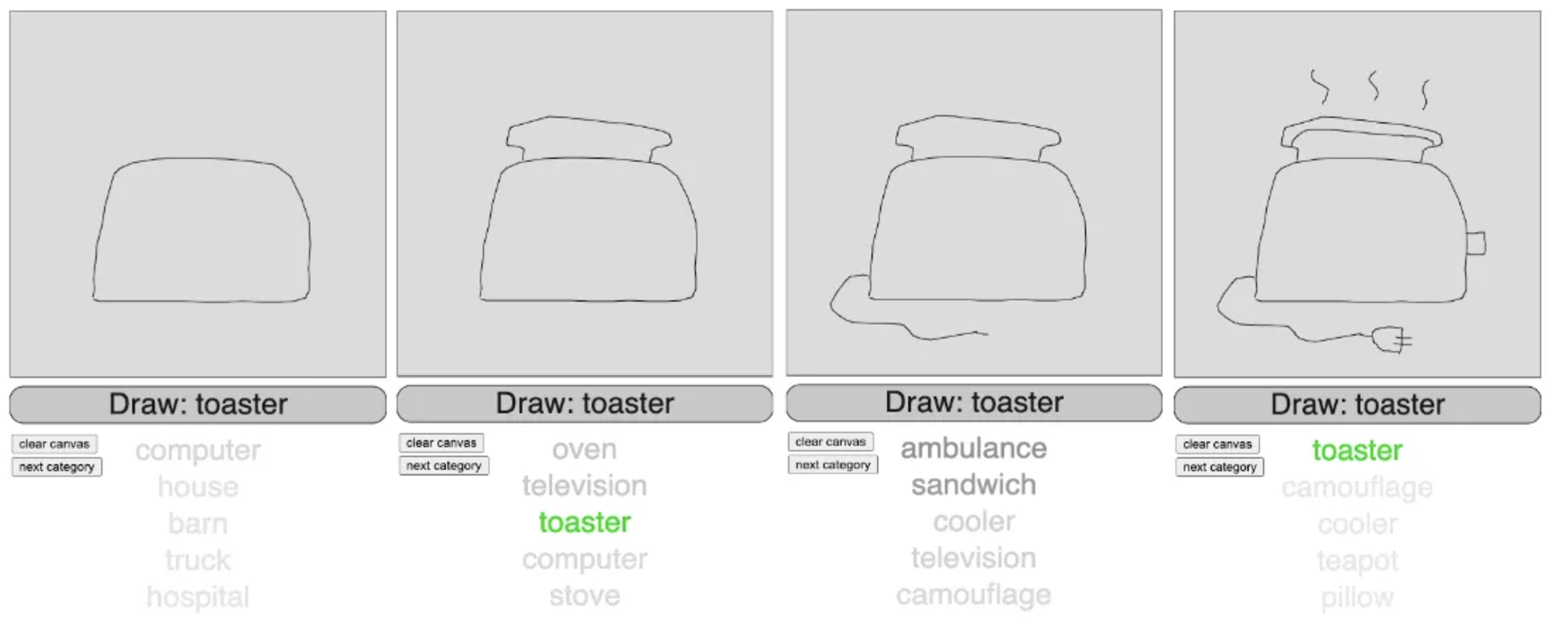
I was more interested in making a demo / test environment than a game per se, so I included the model’s top 5 predictions at each stroke, shaded for confidence. This reveals some of what the model has produced at various stages.
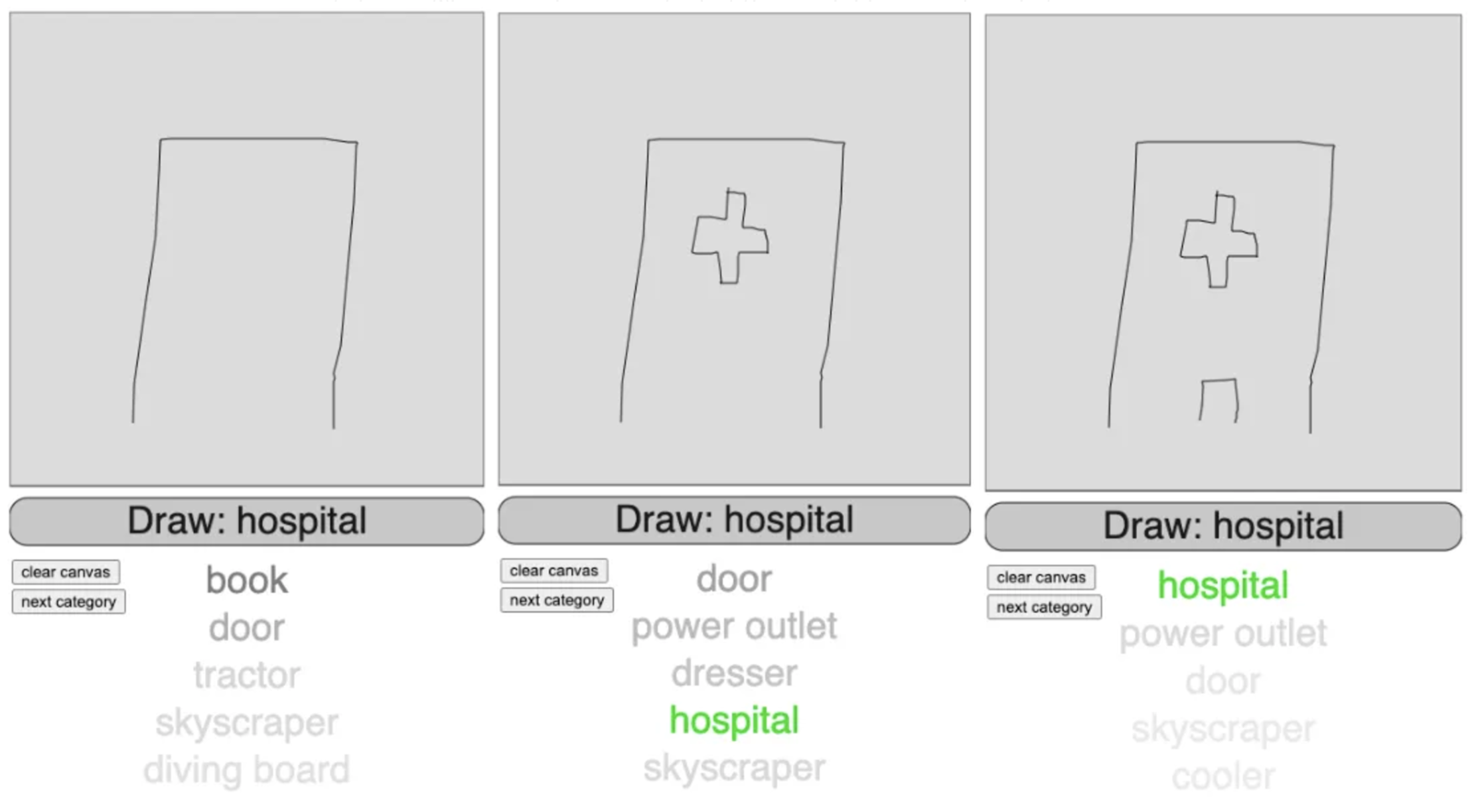
Results#
In most cases the model makes very reasonable predictions, and is often able to make use of key distinguishing features. In the example below, it predicts tractor for the first image with a high degree of confidence. The addition of a rudimentary scoop completely changes things, however, and now the model is very confident in predicting bulldozer.

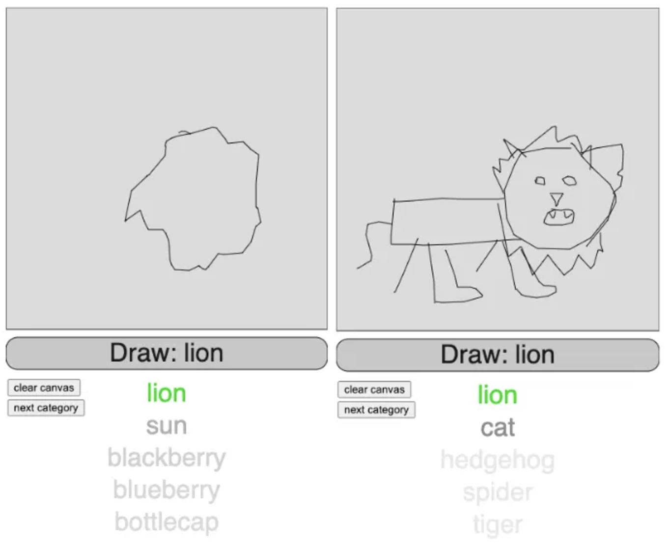
As intended, the model is often able to make good predictions on incomplete drawings. In the first example below, the model correctly predicts lion when given only the outline of a mane. In the second example, I drew the mane last, until which point the model was more likely to predict cat, tiger, or frying pan.
Performance in Javascript is easily fast enough to make predictions on-the-fly, but I did find that the first predict() call to the model ran much more slowly than subsequent calls. This is easily fixed by “warming up” the model with a dummy call on page load.
async function setup() {
    frameRate(30);
    canvas = createCanvas(DRAW_WIDTH, DRAW_HEIGHT + PADDING + INSTRUCTION_HEIGHT + PADDING + FOOTER_HEIGHT);
    background(255);

    console.log('Loading model...');
    model = await this.loadAndWarmUpModel('models/model.json');
    console.log('Model loaded');
}

async function loadAndWarmUpModel(modelPath) {
    const model = await tf.loadLayersModel(modelPath);
    const dummyData = tf.zeros([1, 200, 3]);

    // Warm-up prediction
    model.predict(dummyData).dispose(); // Dispose to free up GPU memory

    return model;
}