Emulating the Apple ][ part 5: ray-tracing in assembly
This is the fifth chapter in an odyssey that encompasses:
- Using test-driven development (TDD) to create an instruction-level simulation of the 6502 microprocessor.
- Reverse engineering the keyboard input and graphics output of an Apple 2 computer (a 1970s computer with the 6502 at its core).
- Combining the pieces into an emulation of the Apple 2 computer accurate enough to run real 1970s software.
- Rewriting the simulation in C++ to make it 500x faster than it was in reality.
- Testing that speed with a ray-tracing graphics engine written in 6502 assembly.
I: First forays in assembly#
After drastically speeding up my 6502 to run at 100s of MHz (instead of the 1Mhz it originally achieved), I found myself wondering what this could enable. What would computer history have looked like, had 8-bit processors reached such speeds in the 1970s? The one way to find out, I thought, would be to try and build something that would have blown an original Apple 2 user’s mind.
This would mean coding in assembly language. Assembly is hard. You are programming at the instruction-level, telling the cpu exactly what to do each clock cycle. It doesn’t help that, in this language, ChatGPT is completely illiterate.
Below you can see a subroutine (essentially a function) that loops over each pixel in a matrix. It is equivalent to the preceding function in Python:
# Python 2D matrix loop

def run():
  for row in rows:
    for col in cols:
      draw_pixel()
; Assembly 2D matrix loop

Run:
        lda #$00
        sta RowCounterAddress
        sta BlockCounterAddress
        sta ThirdCounterAddress

        ForEachRow:
                lda RowCounter
                cmp #MaxRows
                bcs EndRowLoop

                jsr ResetColOffsetIndex

                ForEachCol:                     ; each col is a pixel - 7 per address
                        ; jsr DrawPixel

                        ; Increment col offset index
                        lda Temp2               ; Increment col offset index with carry
                        clc
                        adc #$05
                        sta Temp2
                        lda Temp1
                        adc #$00
                        sta Temp1

                        lda ColCounter
                        clc
                        adc #$01
                        sta ColCounter
                        bcc ForEachCol          ; Hard-coded 256 columns

                AtEndOfRow:
                        ; Increment row offset index
                        lda Temp4               ; Increment row offset with carry
                        clc
                        adc #$05
                        sta Temp4
                        lda Temp3
                        adc #$00
                        sta Temp3

                        ; Reset col counter
                        lda #0
                        sta ColCounter

                        ; Increment row counter
                        inc RowCounter
                        lda RowCounter

                        jmp ForEachRow

        EndRowLoop:
                rts
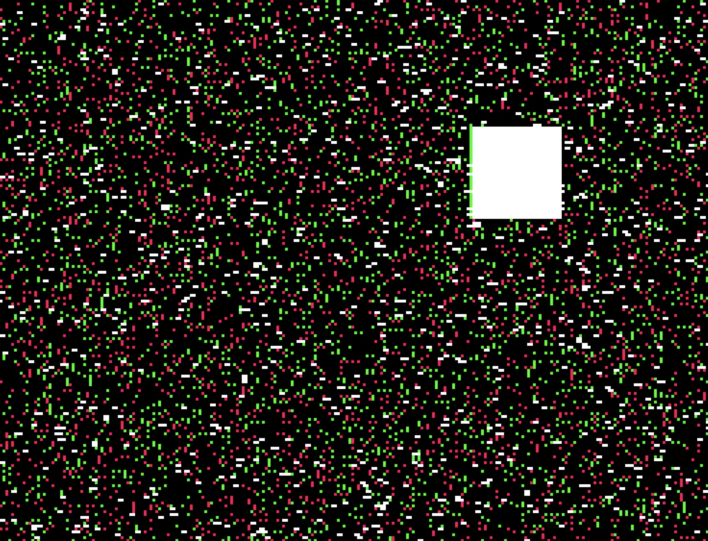
To get a feel for things, I started out trying to get a white square to bounce around in a field of static. This was surprisingly challenging, but I started to get my head around things and decided to raise my ambitions.
II: Towards ray-tracing#
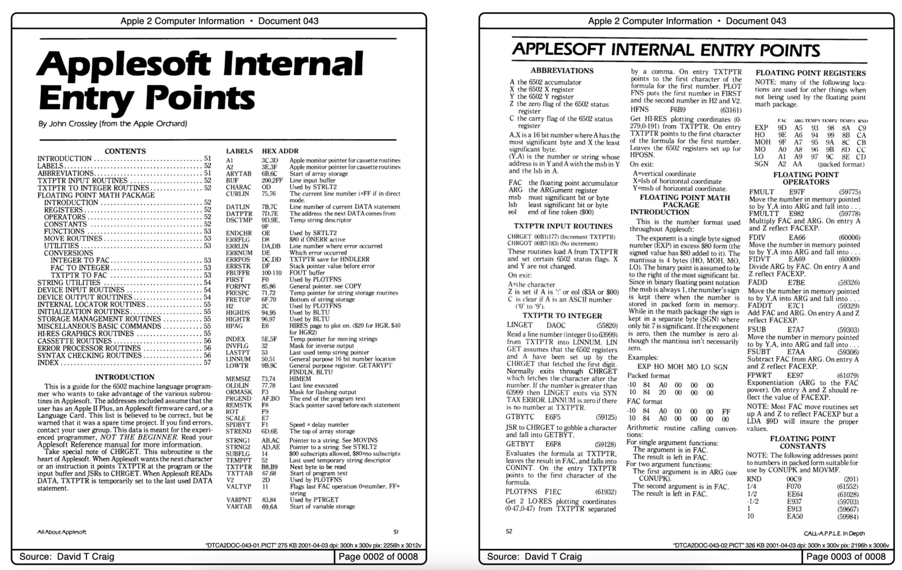
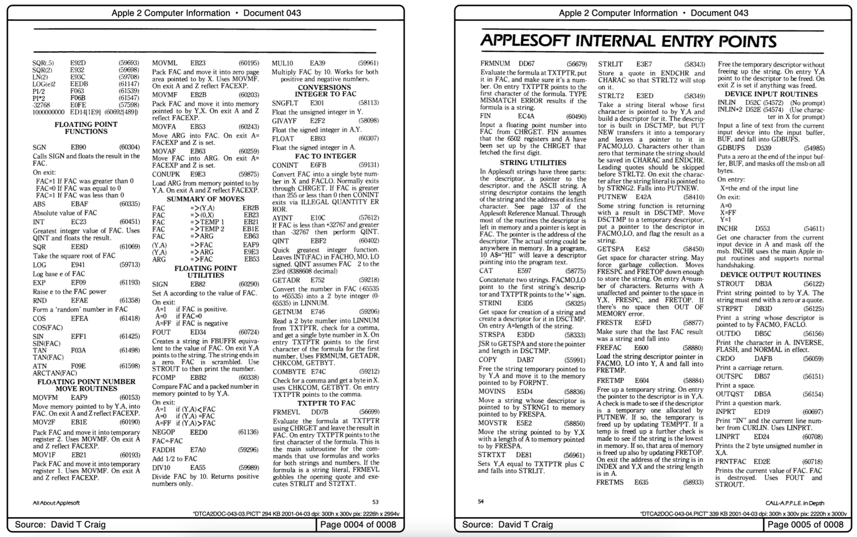
In a previous project, I built a ray-tracing graphics engine, and I wanted to see how hard it would be to get a basic version of it working on the Apple 2. Ray-tracing requires lots of floating-point arithmetic, so I would first need to figure out how to do that.
Later revisions of the Apple 2 included floating point routines in ROM, and these are indeed used by Basic. They are theoretically accessible to the assembly programmer, but I could find no documentation — only this short historic pamphlet, apparently the result of some forensic engineering:
Using these functions is pretty fiddly. To multiply two floats together, you have to do set up some pointers, put some values into memory, and then do something like this:
ldy TempF1High
ldx TempF1Low
jsr MOVMF            ; Pack FAC to address
lda TempF1Low
jsr FMULT            ; Unpack and multiply
ldx TempF1Low
jsr MOVMF            ; Pack
Unfortunately, I found that a lot of these functions work in some unexpected, even misleading, ways. This, for instance, is supposed to be a sine wave:
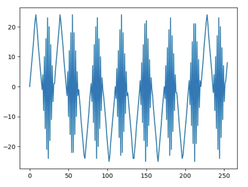
After a lot of testing, I was able to redocument these subroutines and had uncovered enough functionality to do proper floating point arithmetic.
III: A new graphics card#
You’ll remember from chapter 4 that high-res graphics mode is far from ideal for ray-tracing. We want to be able to control every pixel independently, but on the Apple 2 this isn’t really possible. One reason is how much memory it would require — an 8-bit, or 256-value, greyscale bitmap comprising 192 rows of 256 columns would take up 75% of the total addressable space of the cpu. In other words, it’s not practicable.
I solved this problem by inventing my own graphics card standard. It’s very simple, and would have been entirely feasible in the 1970s; it’s just that no-one would have made it because reducing memory usage was far more important than creating simple APIs.
My graphics card is essentially a separate memory bank that holds the 192x256 bitmap, and is accessed by writing to a few memory addresses, exactly how a standard add-on card for the Apple 2 works. To use my graphics card, all you need to do is provide an address and a value. Writing the value triggers the card to put that value in its address.
Now with our imaginary graphics card installed, and using floating point arithmetic, we can draw smooth greyscale images!

Run:
        ; initialise graphics card
        lda #$00
        sta VCARDLOW
        sta VCARDHIGH

        ForEachRow:
                lda RowCounter
                cmp #MaxRows
                bcs EndLoop

                ForEachCol:
                        jsr DrawPixel
                        lda ColCounter
                        clc
                        adc #$01
                        sta ColCounter
                        inc VCARDLOW
                        bcc ForEachCol          ; Hard-coded 256 columns

                lda #0
                sta ColCounter

                inc RowCounter
                inc VCARDHIGH

                jmp ForEachRow

        EndLoop:
                rts
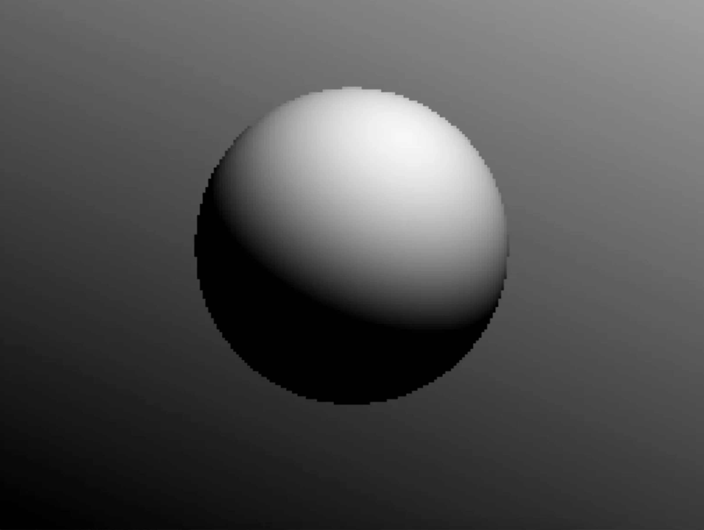
IV: Ray-tracing#
I set myself the goal of rendering a single sphere with a single light source. To start, I prototyped a function in Python and made sure it was as simple as possible. The algorithm goes something like this:
- For each pixel, we fire a ray
- The ray has an origin
- The ray has a direction
- A sphere has a centre
- A sphere has a radius
- Does the ray hit the sphere?
- If it does, where is the point it first hits (not the point it exits)
- What is the normal vector of that point (ie what direction is that point on the sphere facing)?
- How close to the light vector is the normal vector? Or, how much light hits that point on the sphere.
Keen eyes will notice a couple of square root operations avoided. Square roots have a HUGE penalty in this architecture. A single extra square root operation visibly slows things down.
import numpy as np
import matplotlib.pyplot as plt
def ray_sphere_intersection(ray_origin, ray_direction, sphere_center, sphere_radius):
# Convert inputs to numpy arrays for vector operations
O = np.array(ray_origin)
D = np.array(ray_direction)
C = np.array(sphere_center)
r = sphere_radius
# Normalize the direction vector D
# D = D / np.linalg.norm(D) # removing sqrt seems to have no effect
# Compute coefficients of the quadratic equation
a = np.dot(D, D) # 1 if D is normalized - corrects for non-normalised
OC = O - C
c = np.dot(OC, OC) - r**2
b = 2 * np.dot(D, OC)
# Compute the discriminant
discriminant = b**2 - 4 * a * c
# Check for real solutions
if discriminant < 0:
return None
else:
# Compute the two points of intersection t1 and t2
sqrt_discriminant = np.sqrt(discriminant)
t1 = (-b - sqrt_discriminant) / (2 * a)
t1 = (-sqrt_discriminant -b) / (2 * a)
t2 = (-b + sqrt_discriminant) / (2 * a)
# Points of intersection
P1 = O + t1 * D
P2 = O + t2 * D
return {
"t1": t1,
"Point 1": P1,
"t2": t2,
"Point 2": P2,
"normal": C - P1,
}
# Example usage:
ray_origin = [0, 0, 0] # Ray starts at the origin
sphere_center = [0, 0, 5] # Center of the sphere
sphere_radius = 3 # Radius of the sphere
light_vector = np.array([-0.1, 1, 0.2])
# Call the function
pixels = np.zeros((200, 200))
z = 100
for i, y in enumerate(np.arange(-100, 100, 1)):
for j, x in enumerate(np.arange(-100, 100, 1)):
ray_direction = [x, y, z]
intersection = ray_sphere_intersection(ray_origin, ray_direction, sphere_center, sphere_radius)
if intersection != None:
value = np.dot(intersection['normal'], light_vector)
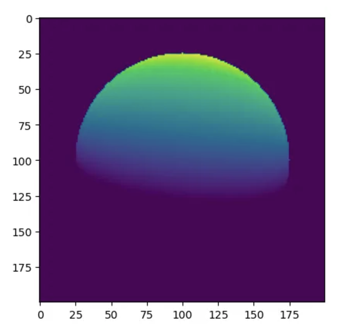
pixels[i][j] = max(0, value)
plt.imshow(pixels)
V: Linear algebra on an 8-bit microprocessor#
This was a real test. For our MVP ray-tracer, we need a few linear algebra operations: we need to add and subtract 3D vectors, and also calculate dot products. Remember that the 6502 can only handle integers between 0 and 255? Floating point numbers are encoded using 5 bytes, using the schema below:
   7       0     31                                  0
  +-+-------+    +-+-------+--------+--------+--------+
  |S|eeeeeee|    |S|mmmmmmm|mmmmmmmm|mmmmmmmm|mmmmmmmm|
  +-+-------+    +-+-------+--------+--------+--------+
 sign exponent  sign        implied-1 mantissa
Each vector comprises three 5-byte floating points. Because the 6502 can only operate on two 1-byte operands at a time, something like a vector addition will take thousands of clock cycles as the component bytes are moved in and out of registers.
Here’s how to calculate the dot product from two vectors in Python:
A = np.array([1, 2, 3])
B = np.array([-1, 0.5, 2])

dot_product = np.dot(A, B)
Here’s the subroutine I wrote to do the same thing in assembly. You’ll notice that this is quite involved, pretty obscure, and, as a novice in assembly, it took me some time.
; All of this code puts pointers to the 2 operand vectors
; into the vector pointers. Because it is a 16-bit
; address space with an 8-bit processor, each vector has
; two pointers, the high 8-bits and the low 8-bits.

; VECTOR ARITH AREA
; Pointers to Vectors
Init:
    V1XHigh = $2400
    V1XLow = $2401
    V1YHigh = $2402
    V1YLow = $2403
    V1ZHigh = $2404
    V1ZLow = $2405

    V2XHigh = $2406
    V2XLow = $2407
    V2YHigh = $2408
    V2YLow = $2409
    V2ZHigh = $240a
    V2ZLow = $240b

    V3XHigh = $240c           ; Where you want the result to get stored
    V3XLow = $240d            ; Might be a whole vector, might be a scalar
    V3YHigh = $240e           ; Consider this space used
    V3YLow = $240f
    V3ZHigh = $2410
    V3ZLow = $2411

    ; LIGHT SOURCE 1 VECTOR3
    Light1XHigh = $20
    Light1XLow = $28
    Light1YHigh = $20
    Light1YLow = $2d
    Light1ZHigh = $20
    Light1ZLow = $32

    ; RAY ORIGIN VECTOR3
    RayOriginXHigh = $20
    RayOriginXLow = $0a
    RayOriginYHigh = $20
    RayOriginYLow = $0f
    RayOriginZHigh = $20
    RayOriginZLow = $14

SetupPointers:
    lda #Light1XHigh
    sta V1XHigh
    lda #Light1XLow
    sta V1XLow

    lda #Light1YHigh
    sta V1YHigh
    lda #Light1YLow
    sta V1YLow

    lda #Light1ZHigh
    sta V1ZHigh
    lda #Light1ZLow
    sta V1ZLow

    lda #RayOriginXHigh
    sta V2XHigh
    lda #RayOriginXLow
    sta V2XLow

    lda #RayOriginYHigh
    sta V2YHigh
    lda #RayOriginYLow
    sta V2YLow

    lda #RayOriginZHigh
    sta V2ZHigh
    lda #RayOriginZLow
    sta V2ZLow

    lda #$25
    sta V3XHigh
    lda #$00
    sta V3XLow

    lda #$25
    sta V3YHigh
    lda #$05
    sta V3YLow

    lda #$25
    sta V3ZHigh
    lda #$0a
    sta V3ZLow

Vector3DotProduct:
    ; Dot Product of Vector pointed to by V1 from Vector pointed to by V2
    ; result left in floating point accumulator as float
    ; uses rest of V3 as temporary storage

    Vector3DotProductX:
        ldy V1XHigh
        lda V1XLow
        jsr CONUPK
        jsr MOVFA

        ldy V2XHigh
        lda V2XLow
        jsr FMULT

        ldy V3XHigh
        ldx V3XLow
        jsr MOVMF

    Vector3DotProductY:
        ldy V1YHigh
        lda V1YLow
        jsr CONUPK
        jsr MOVFA

        ldy V2YHigh
        lda V2YLow
        jsr FMULT

        ldy V3YHigh
        ldx V3YLow
        jsr MOVMF

    Vector3DotProductZ:
        ldy V1ZHigh
        lda V1ZLow
        jsr CONUPK
        jsr MOVFA

        ldy V2ZHigh
        lda V2ZLow
        jsr FMULT

    Vector3DotProductSum:
        ldy V3XHigh
        lda V3XLow
        jsr FADD

        ldy V3YHigh
        lda V3YLow
        jsr FADD
Finally, we could behold ray-tracing on an Apple 2…